Making VGG with PyTorch: Part 3

1. Introduction
2. Building the Model
3. Training the Model
   1. Plan
   2. Loading The Model
   3. Loading The Data
   4. Training
   5. Testing
   6. Evaluation

Plan

The first thing we need to do is make a plan. In our last tutorial we laid out everything we need to perfectly replicate the paper. This blog is about how to replicate the VGG paper, not how to spend hours downloading and figuring out where the ImageNet data set is. In a later tutorial we will look at how to write custom datasets, but not here. The torchvision dataset often does not have the correct ImageNet download address. We may revisit this with ImageNet but for now we will work with something that is easier and we don’t have to deal with that pain. I want this tutorial to be robust and unfortunately that means not using ImageNet.

So instead we will use CIFAR10. This is a large dataset (not as large as ImageNet) but only 10 labels. That will make training a little easier and we will still be able to prove that VGG does what we want it to. This will also help you train on a conventional GPU. So what do we need to change to make this work? Just one line in the model. Our output

# Old last layer
nn.Linear(4096,1000)
# New last layer
nn.Linear(4096,10)

That’s it! (You’ll be surprised how easy this part is of the tutorial)

Loading The Model

This part is so easy I’m just going to show it to you.

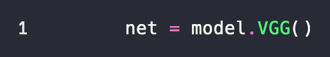
Yeah, that’s it. We just call the class function we made earlier.

Loading The Data

The first thing we need to do is load the data. Torchvision makes this pretty easy. We need a training set and a test set. Torchvision gives us everything we need. See?

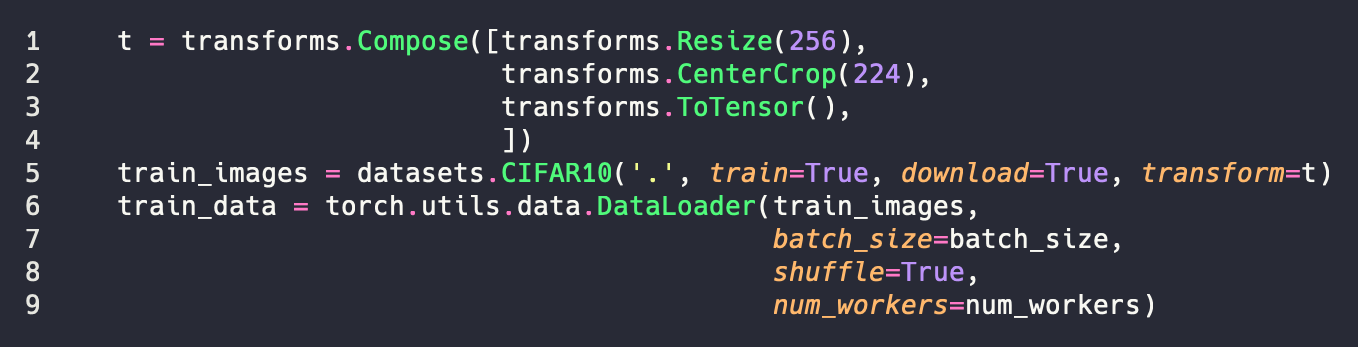
So let’s break this down. First we have our transform t. We can do any set of transforms here by using the Compose function to chain them together. We’re just going to do resize and a center crop here because we know our data is simple and uniform. But we could add things like random rotations and or flips (like we discussed in the previous part). Next, we want to grab the images. Here the first parameter is where we will store the data. We use '.' to select the current directory. We set train=True to tell torchvision that we want the training set. Similarly we pass the transformation set that we want to do. Finally, we create our data loader. The only thing here that should be unknown is the num_workers which is the number of CPU threads we will use to load the data. But we do that when we need the data. Similarly we do the same thing for the test set, but we set train to false.

Training

So now we need to make our training loop. It is fairly simple and we will use our nice python notation to make things readable. Here it is 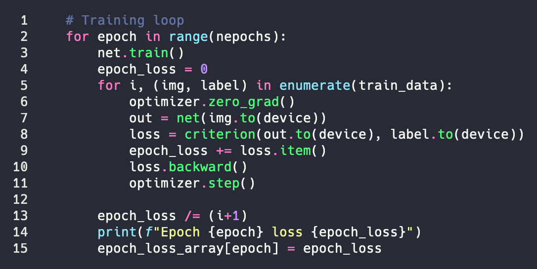We want to set our network to training mode. This is unnecessary since it is the default, but I like to make things explicit. Line 5 is a little odd though. Train data hands us back an image, in the form of a tensor, and a label, which is an integer. In the loop we first reset the optimizer. We send an image (tensor) into our model and see what it passes out. At our first step it is going to be pretty bad. I mean our model hasn’t learned anything yet. So the next step is very important. Here we are telling our model how wrong its guess was. Our backwards step is actually where all the magic happens. If you were programming this without pytorch this would be where you spend all your time. But here it’s just one line. Finally, we take a step in the gradient direction. That’s really it. Our model continues looking at a bunch of images, we tell it how wrong it is, and it tries to use that information to guess better in the future. In this example we are using a simple method. We’re only going to show our model the entire training set N number of times. How ever good it is after that, that’s what we’re going with. But we can come up with other ways to determine how we know when we’re done, such as using a validation set.

Testing

We’re going to do pretty much the exact same thing here.

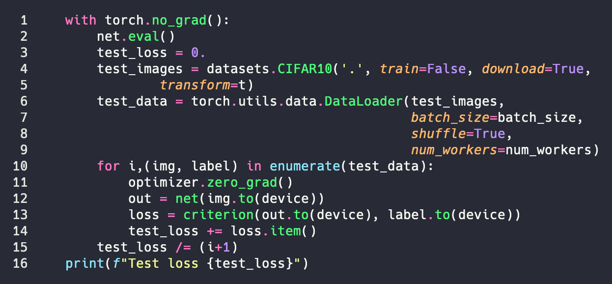
The first thing we do is wrap the test code up with no_grad. The reason we do this is for optimization. We don’t need to keep track of the gradients anymore, this allows us to save memory and speed up the computation a little. The next thing is that we set the model to eval mode. Basically all this does is tells any batchnorm (we don’t use this) and dropout layers (we do use this) to work in evaluation mode. The only other difference is that our loop is smaller because we’re not telling our model how wrong it is. At this point we’ve finished teaching the model and are pushing it out into the real world. Sink or swim time VGG!

Evaluation

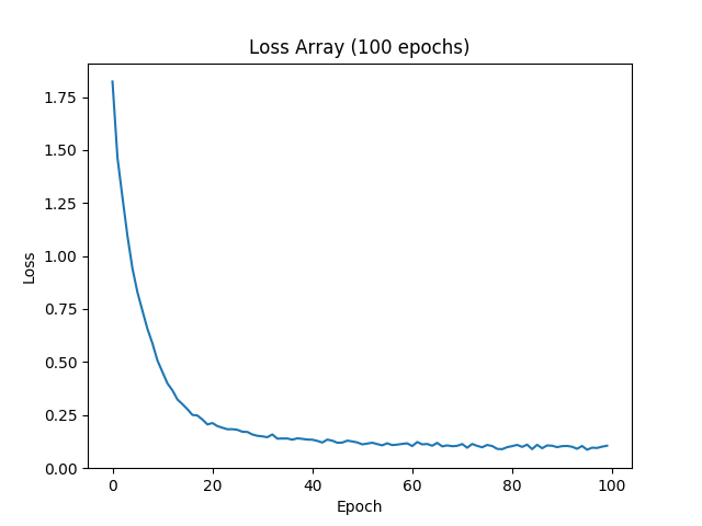
Okay so we got back a test loss of 1.25 and an accuracy of 70%. I mean the VGG paper reports like a 25% error rate. Look at our training loss per epoch!

Time to rejoice, right?

Really this is where our work begins. I know, we built the model, results improved, and we’re doing much better than a coin flip. But this is THE MOST IMPORTANT PART OF THE ENTIRE PROCESS.

It is time to put on our investigator hat and get down to what is going on here.

First, let’s make things approachable to us mere mortals humans. What do our results look like? Let’s select 9 (because it is a nice number) and look at some results.

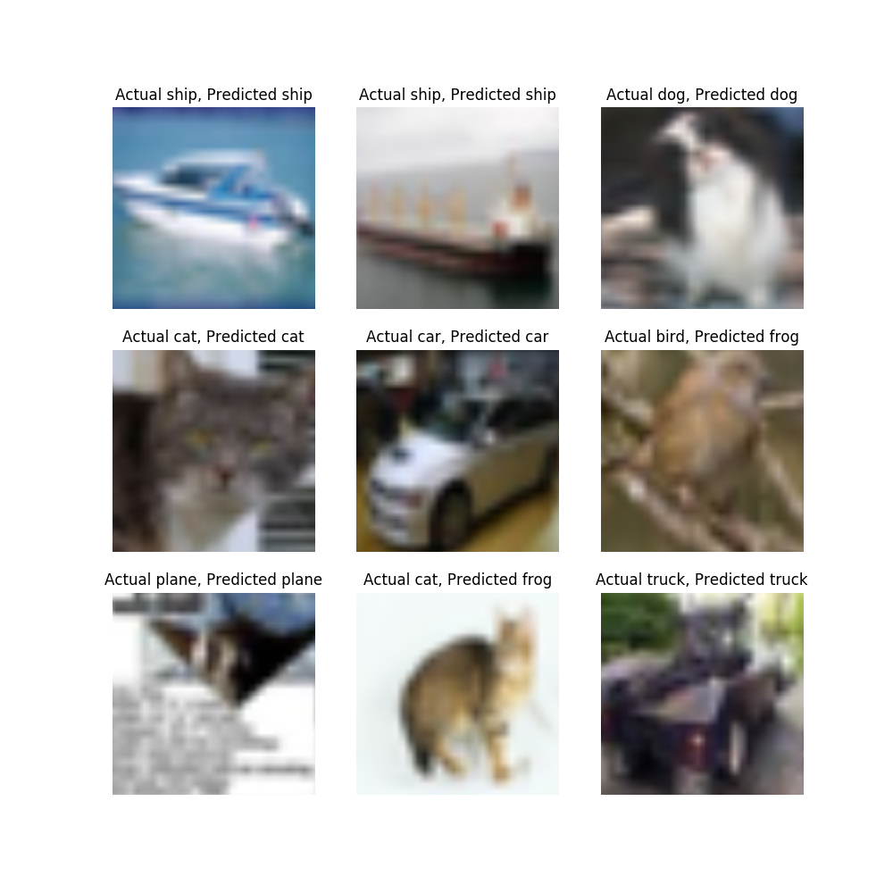
Okay, don’t lie to me. That blob in the upper right is definitely an Otter-Penguin

But we gotta go with the labels. So here we got 7/9. That’s like 80%, pretty good, right? Well we gotta figure out what our model is good at and isn’t. So let’s look at what we did good on and what we didn’t.

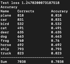
That’s interesting! It isn’t even remotely even. We suck at identifying cats (49%) and are kinda sorta okayish at identifying cars (83%). The first thing I’d do here is ask myself the diversity of the data. But we know CIFAR is pretty good and has even numbers of each instance. So we’re going to skip this, because we already know the answer, but it is a great first thing to ask (this has helped me before and it will help you too!)

So now we gotta ask “When we mess up, HOW do we mess up?” It’s important to remember that you’re always going to mess up. This is normal. We just gotta learn how we have messed up and figure out how to improve. Never give up, never surrender!

So let’s dig deeper. Our worst result was a cat. But does what we misclassified should have been a cat kinda look like a cat? Especially when we’re looking though those blurry lenses!

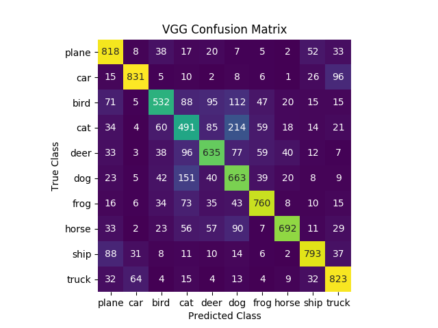
So our cat gives us 49% accuracy (there are 1k examples). The next thing it commonly classifies as is a dog. Dogs kinda look like cats if you squint your eyes enough! I mean my cat sometimes acts like a dog. Close enough. Adding the two together we have 70%. The next thing we classify as a cat is deer! Adding that we’re at 85%! So 85% of our classifications are 4 legged furry creatures! Why is this important? Because a cat looks nothing like a plane. But cats kinda look like dogs. Don’t believe me? QUIZ TIME!

So that 49% isn’t exactly a coin flip. We’re guessing things that are kinda close. Let’s go the other direction. Thinking about the class list we have here, what’s the most distinct objects? We have 10 classes, 4 vehicles (plane, car, boat, truck) and 6 animals (bird, cat, deer, dog, frog, horse). A truck is pretty distinct from a car, boat, plane, and definitely distinct from animals, right? If you agree, it should be unsurprising that trucks score pretty well. So what’s the closes thing to a truck? A car? Well unsurprisingly that’s the most common wrong prediction for a truck. Look even close and we see that vehicles are more likely to be confused with vehicles (cumulative sum of truck as vehicle is 95%) and animals are more likely to be confused with animals (cumulative sum of cats as an animal is 93%). This actually gives us a lot of information about what our model is learning and what it can do!

We’ve learned a few extremely important lessons here.

1) Models are pretty dumb. Don’t trust them more than you would trust a toddler with matches.

2) Models are kinda smart. We can learn from mistakes. We can’t think in binary – right or wrong – but rather a continuum of wrongness.

3) Don’t just accept answers, analyze them. This is also a general principle that applies to life.

4) Don’t treat machine learning like a black box. We don’t just accept answers. We analyze, we question, we iterate.

There’s more that we can go into analyzing our model, but we’re going to call it here for this tutorial. Do you want homework? Try training the model with different number of epochs. Try adding a validation set (how are you going to split your training data? Or test data?) Can you implement the adjusted learning rate from the VGG paper? How does batch sizes change things?

The reason we went through the first two parts was so that we could gain intuition about how to answer these types of questions. Implementing the model is often the easy part. If we don’t have a good understanding of ML and statistics then we are going to have a difficult time analyzing the model. I cannot stress again that analysis is the most important part (it is also the most forgotten part!).

I’ve left my version of the model in a Github so you can see what I did. Try to implement this on your own. Can you figure out the tricks I did in src/model.py?