Making VGG with PyTorch: Part 2

1. Introduction
2. Building the Model
   1. Let’s build
   2. Section 3: Classification Framework
      1. Gradient Descent, Learning Rates, and Mini-batching
      2. Dropout
   3. Pre-Processing
3. Making VGG with Pytorch

This is the second part of a PyTorch tutorial where we replicate the infamous VGG model. In the previous section we focused on a lot of the background and started reading the paper. If you have not read this, I highly suggest it. This part of the tutorial will focus on building the model, as described in section 2 of the paper.

Let’s Build the Model

We now have everything we need to build the model, so let’s do that.

First I’m going to show you what I made, then we’ll talk about each part.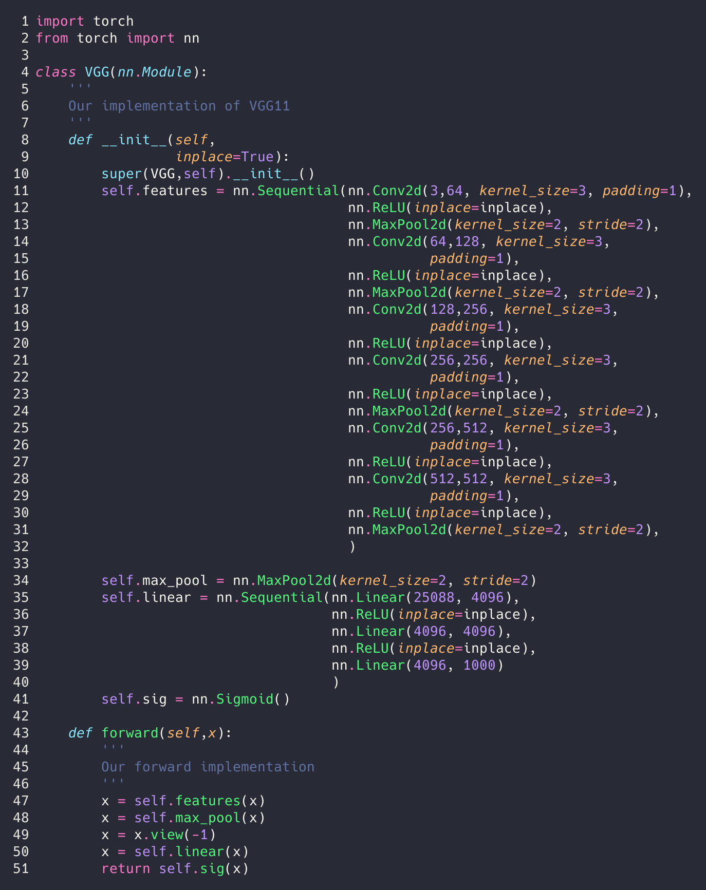

That’s pretty much it. We just followed the column A from the table above. We should note that this is the same thing as was described in section 2.1. The only difference is section 2.1 didn’t tell us exactly where the max pooling layers were.

The key differences we notice in our network and the one from torch are that torch uses a nn.AdaptiveAvgPool2d and we use nn.MaxPool2d. We are just doing what the paper says.

So we understand the paper and what it is asking, but how did we come up with this python code? Let’s start from the top.

Of course we need to import PyTorch (torch). By convention we will also include nn so that we don’t have to constantly type torch.nn.

PyTorch wants us to make our model a class and requires that we have a forward function, which is how the model feeds forward (Side note: we can also add a backward function that would describe how we do back propagation). We inherit the nn.Module class, which contains all the functions that we need. We are just going to overwrite the init and the forward. (If you don’t add a forward definition then your program will complain). Next we create our constructor definition (__init__) and we call super to initialize the parent class first. Next we start making our model!

We use a function called Sequential that does exactly what it says it does. It will take layers and step through them sequentially. We could have similarly wrote

def __init__(self, inplace=True):
    ... 
    self.l0 = nn.Conv2d(3,64, kernel_size=3, padding=1)
    self.l1 = nn.ReLU(inplace=inplace)
    self.l2 = MaxPool2d(kernel_size=2, stride=2)
    ... and so on ...

def forward(self, x):
    x = self.l0(x)
    x = self.l1(x)
    x = self.l2(x)
    ... and so on ...

Sequential gives us a nice way to group parts of our network together, greatly increasing code clarity. Now we need to look at the specifics of what is going on. If you don’t already know what is happening, then it is best to try it out. So let’s see what’s going on. Let’s give it a try.

>>> import torch
>>> from torch import nn
>>> img = torch.randn(3,224,224)
>>> l0 = nn.Conv2d(3,64,kernel_size=3, padding=1)
>>> l0
Conv2d(3, 64, kernel_size=(3, 3), stride=(1, 1), padding=(1, 1))
>>> out = l0(img)
Traceback (most recent call last):
  File "<stdin>", line 1, in <module>
  File "/home/steven/.pyenv/versions/3.7.0/lib/python3.7/site-packages/torch/nn/modules/module.py", line 547, in __call__
    result = self.forward(*input, **kwargs)
  File "/home/steven/.pyenv/versions/3.7.0/lib/python3.7/site-packages/torch/nn/modules/conv.py", line 343, in forward
    return self.conv2d_forward(input, self.weight)
  File "/home/steven/.pyenv/versions/3.7.0/lib/python3.7/site-packages/torch/nn/modules/conv.py", line 340, in conv2d_forward
    self.padding, self.dilation, self.groups)
RuntimeError: Expected 4-dimensional input for 4-dimensional weight 64 3 3, but got 3-dimensional input of size [3, 224, 224] instead
>>> # OH NO!!!! Let's make it 4 dimensions
>>> out = l0(img.unsqueeze(0))
>>> out.size()
torch.Size([1, 64, 224, 224])

Here we create a random tensor of size 3x224x224 to represent our image. That would be the 3 color channels, the width, and the height (PyTorch expects it in this order). We then create a convolutional layer and print it out. You may notice that we are able to actually shortcut some things. That kernel_size=3 is the same as kernel_size=(3,3) (width and height of our kernel). We then send our image through this convolutional layer and we get an error. It is complaining about the input tensor not being 4 dimensions. Weird right? Images are 3D! In PyTorch we expect these objects to be batched together. This is a common technique for speeding up training. So we use the unsqueeze function to expand the tensor and the argument 0 places that 1 in the first position. Now it works fine and we see our output size is 1x64x224x224. So from here we can see that the convolutional layer is changing the size of our color channel. If we remember back to the paper they mention that they used a padding of 1 to ensure the size is the same. So convolutions change the size of input tensors, right?

>>> test_layer = nn.Conv2d(3,64,kernel_size=3)
>>> test_out = test_layer(img.unsqueeze(0))
>>> test_out.size()
torch.Size([1, 64, 222, 222])

That’s EXACTLY right! We added this padding of 1 pixel all around the image so that we would preserve the size. Now let’s continue with our test coding.

>>> l1 = nn.ReLU()
>>> out1 = l1(out)
>>> out1.size()
torch.Size([1, 64, 224, 224])
>>> l2 = nn.MaxPool2d(kernel_size=2, stride=2)
>>> out2 = l2(out1)
>>> out2.size()
torch.Size([1, 64, 112, 112])

So here we learned that ReLUs don’t modify the size of our input while MaxPools halve them (test with other inputs, it isn’t always half!). Similarly we apply linear layers.

Now moving to the forward function this all probably looks straight forward except for the view command. Before this we were working with tensors, but linear layers don’t accept tensors as input, they accept vectors (to the math nerds complaining: I don’t care). By using this view command we are converting our object into a single vector and then passing it into our linear layers. You may be asking yourself, why “25088”? Well that’s because our output from the max pool is 1x512x7x7. The 4096 was chosen by the researchers and tested to be a good fit, while the last thousand is the number of objects we are trying to classify.

That’s it! We have our model. Now onto the tricky part.

Section 3: Classification Framework

You know the drill. Read it first.

Okay there’s a lot here, don’t get discouraged. This is the hardest section to read through. There’s a lot of important stuff so let’s try keeping track of what is said here. But the section is well written and makes it possible for us to replicate the results.

The first thing we run into is that we’re using a mini-batch gradient descent with momentum. We’re then told that the batch size is 256 and momentum is 0.9 (having the hyper parameters is really helpful in trying to reproduce results!). We get the regularization and hyper parameter, we get that there are dropout layers and where they are (remember the difference in our model and PyTorch’s?). They then tell us that they adapt the learning rate, first starting at \(10^{-2}\) then decrease by a magnitude when the validation accuracy stops improving (and that it happened 3 times). We finally see that they ran a total of 370k iterations for a total of 74 epochs. They then wrap up this dense paragraph with a conjecture about how depth over breadth of networks helped them converge in a smaller number of epochs and that their pre-initialisation helped.

That’s a pretty dense paragraph. Let’s stop reading here and do some coding. We have most of what we need here to replicate VGG and we still have a lot to talk about PyTorch.

First, let’s update our model real quick. We need to incorporate the dropout layers that they told us about.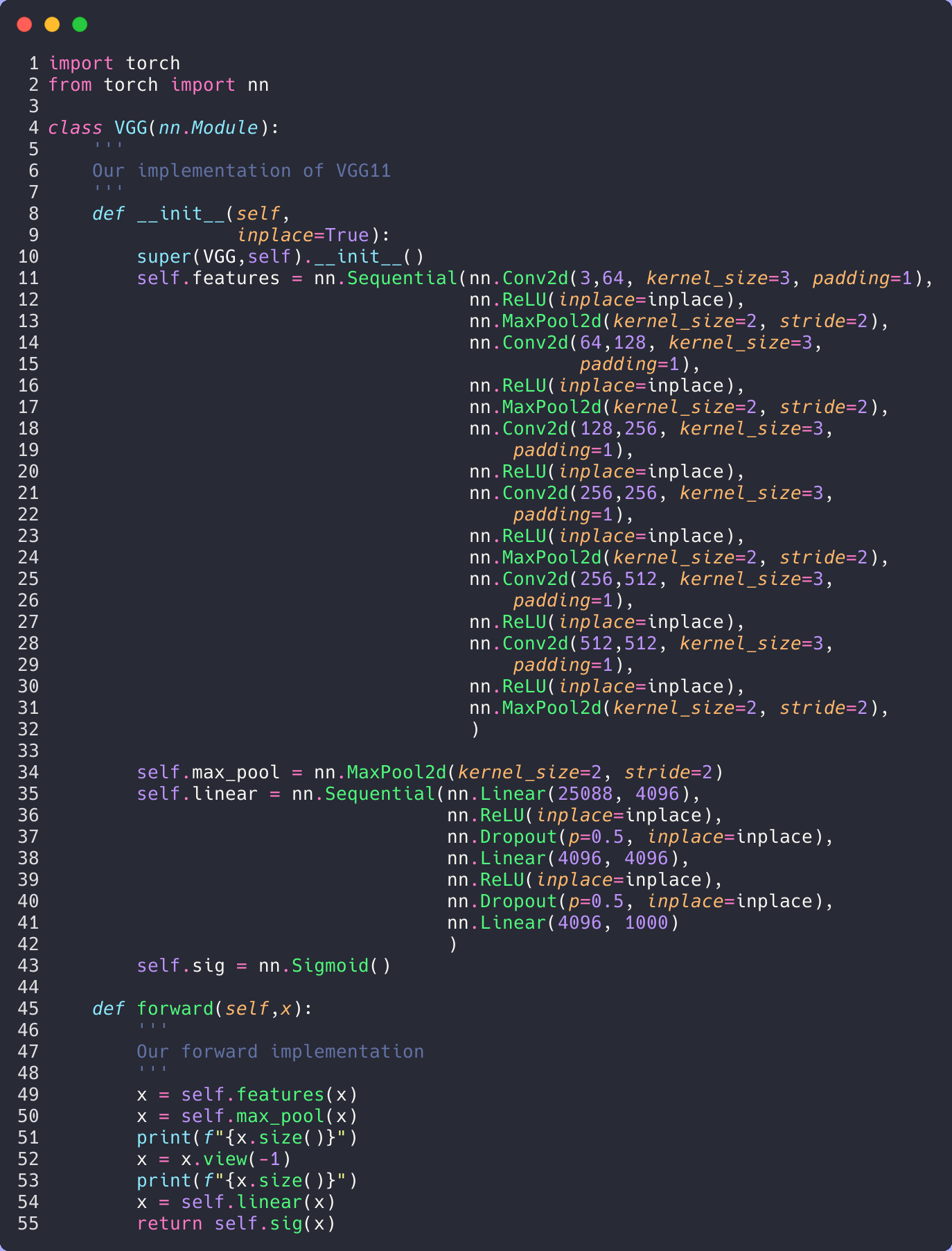

Let’s break down that paragraph a little bit.

Gradient Descent, Learning Rates, and Mini-batching

In machine learning a single pass through all our data is called an epoch (pronounced e-pək, like “epic”). Then we do our back-propagation with some form of a gradient descent (finding a minima to our problem). This is one of the most expensive parts of our algorithm. The following image shows a few different gradient descent algorithms (Adam, or variants of it, is the most widely used right now). 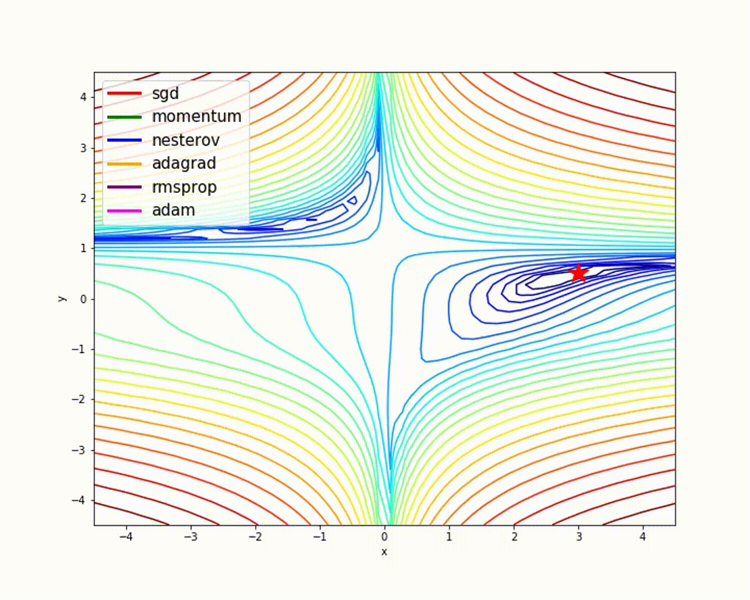In this paper we are using the standard stochastic gradient descent (torch.optim.SGD). SGD has a momentum component (see the green path above?), and that is the parameter they are setting to 0.8.

Side note: Though Adam is the most commonly used, it isn’t always the best for the task. You may notice that momentum is very fast, same with (Nesterov aka NAG). The improvement that Adam has is that it doesn’t deviate as much as NAG or Momentum, meaning it is less likely to become trapped in a local optima. I encourage you to investigate these algorithms more and play around with them. The best tool to use depends on your solution space.

Now let’s look at the equation for basic gradient descent.

\[a_{n+1} = a_n - \gamma\nabla F(a_n)\]

What this says is that there’s some function \(a_n\) that is dependent on a previous iteration, \(a_{n-1}\) The difference between these two is that we subtract a gradient of the function during each iteration \(\nabla F(a_n)\). The term \(\gamma\) here is our step-size, which in machine learning we call the “learning rate”. If \(\gamma\) is small, then we step towards the minima slower BUT we are less likely to fall into a local minima. Think about if you are hiking outside. Larger steps will make your hike faster, but you are more likely to twist an ankle. In sections of the hike where the path is more dangerous you slow down and take smaller and more careful steps. In machine learning we want to apply the same idea. If we have lots of local minima (this may be unknown!) it is safer to take smaller steps (set \(\gamma\) to be smaller). If we know we have a nice solution space then we can run (set \(\gamma\) to be relatively large) without risk of danger. In the VGG paper they do a combination of this. They start off running and then slow down as they get closer to their final destination. This is a good trade-off and allows for fast and accurate training, but comes with some assumptions (a topic for another time).

Now that we (kinda) understand back-propagation we want to speed it up. One way to do this is to group together (batch) some of our training dataset and do this gradient descent all at the same time. Not only does this speed things up, but actually makes the algorithm more robust and helps us avoid local minima. It is not uncommon for these batches to be in powers of 2, but this is not a requirement. One drawback of a large batch size is that it requires more memory. So if you are running out of memory, maybe decrease your batch size appropriately (there are other things you can do to reduce memory consumption, but we’ll save that for another time).

Dropout

Dropout is a training layer, in that it only affects training. Essentially we create a probability that a neuron is going to get ignored. This reduces the effect of a single neuron, meaning that one doesn’t dominate, and thus can help prevent over-fitting.

Pre-processing

Now that we got through that really dense paragraph we can move on. The next paragraph talks about initializing the network. In this tutorial we will ignore this because PyTorch (and other frameworks) handle this step for us. Reading on we begin to understand how the authors pre-processed their data. This is one of the most important aspects of machine learning. There is a common phrase “garbage in, garbage out”. It is important to remember that machine learning algorithms are not magical and don’t think like we humans do (or really any animal). There are many examples where bad training data resulted in bad results. Let’s talk about one.

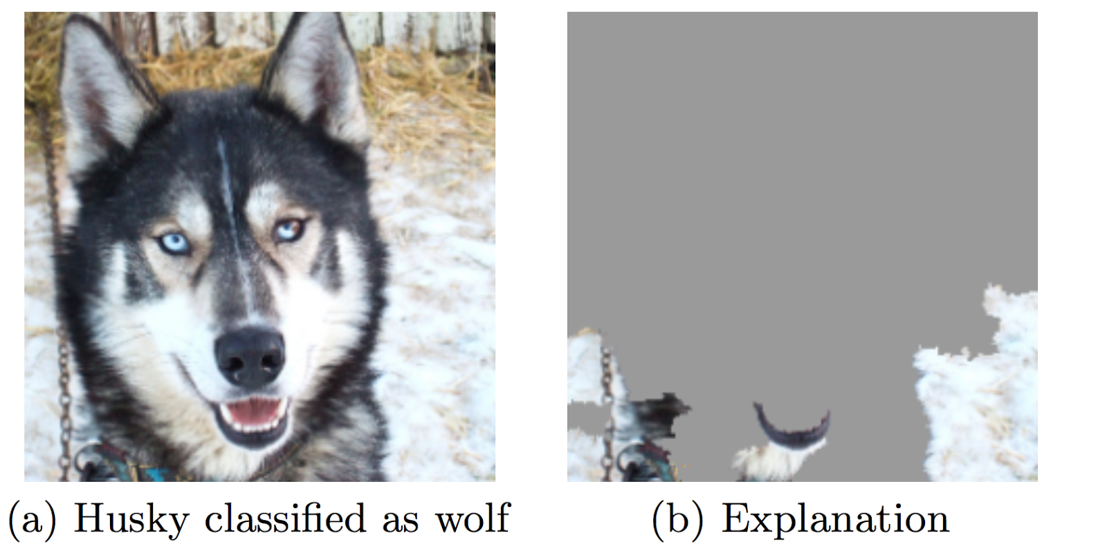
Researchers at the University of Washington developed a model trying to classify Wolves and Eskimo Dogs (huskies). In this they carefully selected images such that wolves always had snow in the background while huskies did not. By doing this they were able to always create adversarial examples where any husky that had snow in the picture was classified as a wolf. The paper focuses on developing an algorithm to explain classifications.

The thing to remember is that the algorithm will find the best way to solve the specific task you give it. There’s careful wording there. I didn’t say “the task you want it to solve” I mean “the task you give it.” I’ll leave you with small comic to illustrate this point.

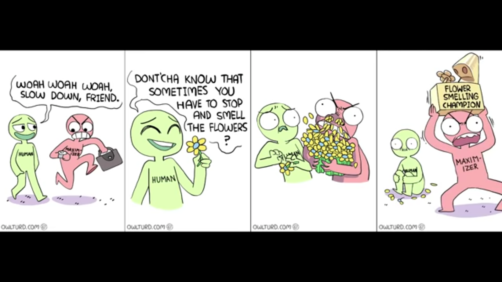
Clearly we don’t intend the maximizer to literally smell the flowers. But since that is what we told it to do, that is what it did. This comic is taken from Robert Miles’s YouTube where he discusses this topic in depth. I encourage you to check them out.

Now back to the paper. We see that they use a fixed size for the images, 224x224. This both helps reduce the memory consumption, smaller images require less memory, and means their input layer can be static/isn’t padded with zeros (don’t worry about this). The important part is that they say that they do a random cropping of the rescaled images, random horizontal flipping, and random RGB color shift. This may seem odd. All these things create slight differences in the photos and thus attempt to make the only relevant feature in the image the object we are interested. (Imagine if we collected a bunch of photos of fish. It wouldn’t be surprising if many of those photos had human hands holding the fish or a fishing rod was somewhere in the picture) Flipping the image reduces the likelihood of orientation becoming a distinguishing feature (such as if all our pictures of dogs happened to be looking right). RBG color shifts can help with factors such as lighting (try to think of others).

Let’s look at a quick example. I pulled a random image out of ImageNet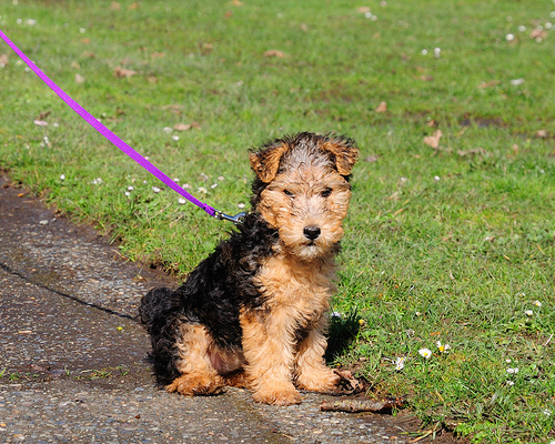

This image is originally 400x500. In ImageNet not all the images are the same size or shape, so resizing will almost always be an included pre-processing step.

We follow the pre-processing steps in the VGG papger, so we scaled the image to 256x256, applied a random cropping (shrinking the image to 224x224), a random horizontal flip, and then color jitter (with brightness, contrast, and saturation set to 2. There was no special meaning behind this, just a random choice). Here are 5 example images showing the transformations. Note that many of these transforms are random, that is why we are applying it 5 different times to the same image, so we can clearly see the effect of each transform.

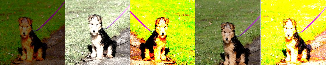
We can still tell that there is a cute little puppy in all the images, but things are different. Maybe this pre-processing is good, maybe it isn’t. There is still a leash in the picture (looking at several ImageNet pictures of dogs, leashes are common! This could mean a leash is an accidental identifier, like snow). But we can tell that we are getting some of the effects that we want. The puppy is no longer always centered in the image, the texture is sometimes washed away (including the grass), and we don’t have a direct color dependency. These things will help our network better generalize. As you can imagine, this is why a big part of the job of machine learning and data science is pre-processing and editing these images. Intuition is very helpful here, but you will only gain that with experience. But that’s why we’re here right? To learn.

That’s about it. There’s more details in the paper, but this is what we need to get building. So let’s do it!