Making VGG with PyTorch: Part 1
Table of Contents
I often see tons of tutorials for PyTorch that I often find wanting. Things aren’t explained and we don’t get a clear picture of how to use the tools we have or understand the decisions that we are making. So to add to the countless tutorials around I’m going to try something different. We’re going to read a paper and try to replicate the results. We will build everything from PyTorch and see how well we can do. Because of this, we’re not going to be as quick as most tutorials, but hopefully the reader is left with a better understanding of the material. Hopefully by the end of this tutorial the reader will be able to read a machine learning paper and be able to replicate the model. In this tutorial we are assuming that the reader is not familiar with PyTorch nor with machine learning. We will be covering a lot of material here, some will be basic, and others will be more advanced. Feel free to skip over sections as needed. This material is not substitute for a course in machine learning and we will even be avoiding extremely important topics (such as back-propagation) that PyTorch abstracts away for us. The focus of this paper is replication, not understanding the material in depth. This is just the minimum needed to replicate this paper.
What you need:
- A computer
- Python3 and PyTorch
- The ability to read
- Your critical thinking cap
Great! Now that we got all this, grab this paper. This is the infamous VGG paper, and we will be going through, reading, and then implementing it. Like any good research, replication is key. If your readers can’t replicate your paper, you need to write better.
But first
Let’s make sure that we have a baseline and know what we’re doing.
>>> # Load models from torchvision
>>> from torchvision import models
>>> # Let's see what models exist
>>> models.__dir__()
    ['__name__', '__doc__', '__package__', '__loader__', '__spec__', '__path__',
    '__file__', '__cached__', '__builtins__', 'utils', 'alexnet', 'AlexNet',
    'resnet', 'ResNet', 'resnet18', 'resnet34', 'resnet50', 'resnet101',
    'resnet152', 'resnext50_32x4d', 'resnext101_32x8d', 'wide_resnet50_2',
    'wide_resnet101_2', 'vgg', 'VGG', 'vgg11', 'vgg11_bn', 'vgg13', 'vgg13_bn',
    'vgg16', 'vgg16_bn', 'vgg19_bn', 'vgg19', 'squeezenet', 'SqueezeNet',
    'squeezenet1_0', 'squeezenet1_1', 'inception', 'Inception3', 'inception_v3',
    'densenet', 'DenseNet', 'densenet121', 'densenet169', 'densenet201',
    'densenet161', 'googlenet', 'GoogLeNet', 'mobilenet', 'MobileNetV2',
    'mobilenet_v2', 'mnasnet', 'MNASNet', 'mnasnet0_5', 'mnasnet0_75',
    'mnasnet1_0', 'mnasnet1_3', 'shufflenetv2', 'ShuffleNetV2',
    'shufflenet_v2_x0_5', 'shufflenet_v2_x1_0', 'shufflenet_v2_x1_5',
    'shufflenet_v2_x2_0', '_utils', 'segmentation', 'detection', 'video']
>>> # Load the model
>>> vgg = models.vgg11()
>>> # Let's see what it looks like
>>> vgg
VGG(
  (features): Sequential(
    (0): Conv2d(3, 64, kernel_size=(3, 3), stride=(1, 1), padding=(1, 1))
    (1): ReLU(inplace=True)
    (2): MaxPool2d(kernel_size=2, stride=2, padding=0, dilation=1, ceil_mode=False)
    (3): Conv2d(64, 128, kernel_size=(3, 3), stride=(1, 1), padding=(1, 1))
    (4): ReLU(inplace=True)
    (5): MaxPool2d(kernel_size=2, stride=2, padding=0, dilation=1, ceil_mode=False)
    (6): Conv2d(128, 256, kernel_size=(3, 3), stride=(1, 1), padding=(1, 1))
    (7): ReLU(inplace=True)
    (8): Conv2d(256, 256, kernel_size=(3, 3), stride=(1, 1), padding=(1, 1))
    (9): ReLU(inplace=True)
    (10): MaxPool2d(kernel_size=2, stride=2, padding=0, dilation=1, ceil_mode=False)
    (11): Conv2d(256, 512, kernel_size=(3, 3), stride=(1, 1), padding=(1, 1))
    (12): ReLU(inplace=True)
    (13): Conv2d(512, 512, kernel_size=(3, 3), stride=(1, 1), padding=(1, 1))
    (14): ReLU(inplace=True)
    (15): MaxPool2d(kernel_size=2, stride=2, padding=0, dilation=1, ceil_mode=False)
    (16): Conv2d(512, 512, kernel_size=(3, 3), stride=(1, 1), padding=(1, 1))
    (17): ReLU(inplace=True)
    (18): Conv2d(512, 512, kernel_size=(3, 3), stride=(1, 1), padding=(1, 1))
    (19): ReLU(inplace=True)
    (20): MaxPool2d(kernel_size=2, stride=2, padding=0, dilation=1, ceil_mode=False)
  )
  (avgpool): AdaptiveAvgPool2d(output_size=(7, 7))
  (classifier): Sequential(
    (0): Linear(in_features=25088, out_features=4096, bias=True)
    (1): ReLU(inplace=True)
    (2): Dropout(p=0.5, inplace=False)
    (3): Linear(in_features=4096, out_features=4096, bias=True)
    (4): ReLU(inplace=True)
    (5): Dropout(p=0.5, inplace=False)
    (6): Linear(in_features=4096, out_features=1000, bias=True)
  )
)
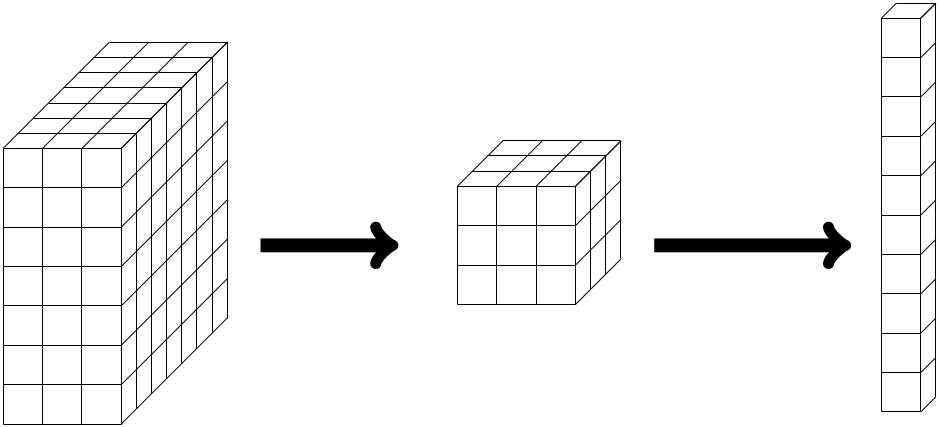
Okay, so what did we do here. We kinda knew that Torch already had common models installed, and with VGG being so common we knew it would be here. So we looked at what models we have and decided to set select the vgg11 model. Then we just printed it out. We can see that there are three main sections to this model. There is the features section, the average pooling, and the classifier. For now let’s think about it like this picture. We’ll start breaking this down later.
We can access each of these parts individually, for example we can see features by typing vgg.features. We can also see each layer, for example we can see the very first layer of features by typing vgg.features._modules['0'].
Okay, so we have an example model, and we know how to access and modify the existing models. That’s good, and important, but let’s try to make this on our own. If we read through the paper and end up making something different we know there’s a mistake. Pretty much we have the answer in the back of the textbook but our professor isn’t going to give us credit unless we can show our work. This is only good to verify.
Let’s Get Reading
We always start with the abstract. It tells us what the problem is, how the authors solved it, and their results. A good abstract tells us if a paper is useful to us or not. I’m going to completely copy it here for reference.
1
2
3
4
5
6
7
8
9
10
11
12
In this work we investigate the effect of the convolutional network depth on its
accuracy in the large-scale image recognition setting. Our main contribution is
a thorough evaluation of networks of increasing depth using an architecture with
very small (3x3) convolution filters, which shows that a significant improvement
on the prior-art configurations can be achieved by pushing the depth to 16-19
weight layers. These findings were the basis of our ImageNet Challenge 2014
submission, where our team secured the first and the second places in the
localisation and classification tracks respectively. We also show that our
representations generalise well to other datasets, where they achieve
state-of-the-art results. We have made our two best-performing ConvNet models
publicly available to facilitate further research on the use of deep visual
representations in computer vision.
So the key takeaways here we should see is that:
- VGG was built to perform image recognition tasks
- We use “very small” convolution filters, sized 3x3
- Depth is important
- The model is convolutional
- The model produced state of the art results in 2014
Looks like we got everything we wanted from the abstract. Looking back at the above model, we see in fact that every convolutional layer does indeed have a 3x3 filter.
Let’s keep reading. Read the introduction. Don’t worry, I’ll wait. Seriously, read it!

Okay so we see some brief introduction to the problem and some references to other works (more to read!). We also see that the main part of this research is about the dept of the convolutional network and experimenting with that (remember, AlexNet only came out in 2012. We’ve come a ways since then. This being one of the important papers). So the authors say “…which is only feasible due ot the use of very small (3 x 3) convolution filters in all layers”. The date here is important because we were (are) still limited by the GPU memory. Continuing, we see that VGG is able to accomplish different visualization tasks. Finally we find out how the paper is organized, i.e. what we need to read. We see that the model is described in section 2 and in section 3 the authors describe their training and evaluation. These will be the most important parts to us.
Section 2
Let’s read it before we continue 
We look for graphs and tables first when reading, right? 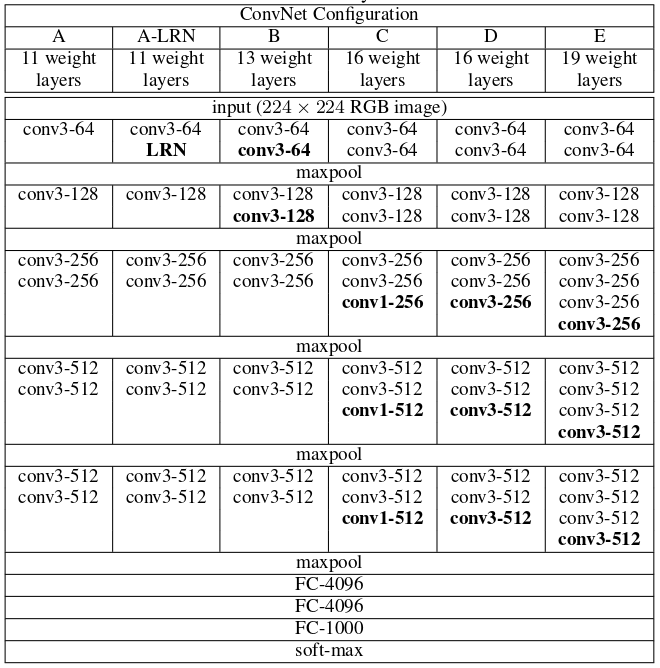
Looking at column A we can see a pretty simple 11 weight network. We can imagine it looking like this.

We can see that the network isn’t very wide but it is deep. This may not seem like innovative work, but let’s remember the universal approximation theorem. If we recall, with a single hidden layer we can approximate any function. But importantly, in that theorem, we may have to have an extremely wide network to make that approximation. We’ll note here that our network isn’t very wide. That’s an importance to this paper, that the breadth is traded for depth.
So reading this section we note some important things about the network. We learn that for preprocessing they minus the mean rgb value (from the training set). We also find that padding is used to preserve the image size through convolution layers and that stride is always 1. The max pooling has a window of size 2x2 and a stride of 2, meaning we’re going to halve the image size each time. The authors tell us that finally there are two fully connected linear layers sized 4096 and a final one of size 1000, to match the number of classified objects in the dataset. We also find that the layers are connected with ReLU activations.
There’s more discussion about wide vs dept networks and this is an important topic that the reader should learn about, but is not necessary for replicating this paper.
But to build the model we see 4 main objects that we need to understand. There’s convolutional layers, ReLUs, MaxPooling, and Fully Connected layers. Let’s look at what these are before we move on.
Linear Layers
We’re going to start with Linear Layers because they are easier to understand and will help us understand convolutional networks. Your reading about neural networks, machine learning, black magic, and deep learning have most likely been referring to fully connected neural networks. They look like this.
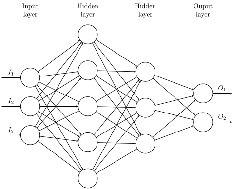
This model has an input layer, 2 hidden layers, and then an output layer. This network is considered deep because it has \(\geq\) 2 hidden layers. The reason for this distinction is because of that universal approximation theorem mentioned above. It states that if we have a sufficiently wide, but finite, single hidden layer, we can approximate any continuous function on compact subsets of \(\mathbb{R}^n\). One of the defining points of the VGG paper that we’re reading is that we can also use a sufficiently deep network and get better performance. We trade breadth for depth.
Okay, back to linear layers. Each of these nodes in the diagram represents a point of data, some number. Each of these numbers are connected to each number in the following column. The math here is fairly simple. We’ll say that each neuron has some value \(x\) and each line connecting them has some weight \(w\) and each layer has some bias \(b\). We can then get the feed forward function by doing \(<w,x> + b\) (the standard inner product).
A linear feed forward network is that easy! You have some data, you do a little inner products, a little addition, and presto! You got an answer.
A very naive implementation of this network in PyTorch would look like this:
1
2
3
4
5
6
7
8
9
10
11
12
import torch
from torch import nn

class nn(nn.Module):
    def __init__(self):
        super(nn, self).__init__()
	# nn.Linear(number of nodes coming in, number of nodes being connected to)
        self.layers = nn.Sequential(nn.Linear(3,5),
                                    nn.Linear(5,3),
                                    nn.Linear(3,2))
    def forward(self, x):
        return self.layers(x)
This wouldn’t produce very good results without the other features we’re going to talk about, but this would work.
Of course we have to train the network. We’re not going to talk about back propagation in detail within this tutorial because PyTorch abstracts that away for us, but I highly encourage every reader to read about it and make sure that they understand gradient descent. Understanding gradient descent is the key to back-prop and will help you better train your networks. Please read up on back-prop. You cannot be a machine learning expert if you do not understand this concept.
ReLU
The next easiest thing to understand is ReLU. A lot of the inspiration for neural networks comes from how brains operate. One defining feature is that neurons are kinda like capacitors. Stimulus causes charge to build up on one side and then once enough charge is built up the neuron fires. This is called an action potential. We simulate that in neural networks with things called activation functions. The classic activation function is called the Sigmoid Function \((\frac{1}{1+e^{-x}})\). This function has an \(x\) range of \([-\infty,\infty]\) but a \(y\) range of \([-1,1]\). Essentially we are creating an on and off switch for our networks. We can think of it this way because close to the origin the sigmoid function is very steep. There’s a whole class of activation functions that can be used. Some people even use the step function, which literally is an on/off switch. One of the bigger breakthroughs in machine learning is the ReLU (pronounced like Ray-Lou). ReLU is simpler than the sigmoid function. It is simply \(\max(0,x)\). We can compute that extremely fast. Sigmoid is a little hard to calculate because of the exponential function. Previous to ReLU it was thought that we needed a smooth and continuous function. Turns out we don’t! There’s other functions that are basically smooth and continuous alternatives to ReLU that are becoming popular, but it is good to know the history.
For PyTorch we may want to adjust the previous network to look like this
1
2
3
4
5
6
7
8
9
10
11
12
13
14
import torch
from torch import nn

class nn(nn.Module):
    def __init__(self):
        super(nn, self).__init__()
        self.layers = nn.Sequential(nn.Linear(3,5),
				    nn.ReLU(),
                                    nn.Linear(5,3),
				    nn.ReLU(),
                                    nn.Linear(3,2),
				    nn.ReLU())
    def forward(self, x):
        return self.layers(x)
Convolutional Layers
Now for the big one! A convolutional layer is a lot like a linear layer. A big difference is that with linear layers we are working with vectors of data, but in convolutional networks we are working with tensors. A convolutional network is extremely popular in graphics because with images there are spacial relations. Images are essentially 3-tensors composed of color channels, widths, and heights. A single channel (grayscale) image would just be a matrix of pixel values. In a convolutional network what we do is take a “kernel” and slide it over the input tensor (image). Let’s see what this looks like.
If we look at the first step of the red filter we see that we can get \((0)(-1) + (0)(-1) + (0)(1) + (0)(0) + (1)(156) + (-1)(155) + (0)(0) + (1)(153) + (1)(154) = 158\) So we’re just doing an inner product with the kernel and the windowed region on our tensor. Neat! It is pretty simple.
There’s one equation to remember with convolutional networks. \(\frac{W-K+2P}{S}+1\) That’s the size (width or height), the kernel size, 2 times the padding, divided by the stride length and plus 1. That results in the size of resulting tensor. Notice how if we let \(k=3, P=1, S=1\) that the output is \(W\). You bet we’re going to use that.
In PyTorch we can implement a convolutional layer similar to the linear layers.
1
2
3
4
5
6
7
8
9
10
11
12
import torch
from torch import nn

class nn(nn.Module):
    def __init__(self):
        super(nn, self).__init__()
	# nn.Conv2d(number of input channels, number of output channels)
        self.layers = nn.Sequential(nn.Conv2d(3, 64, kernel_size=3),
                                    nn.Conv2d(64, 64 kernel_size=5),
                                    nn.Conv2d(64, 100 kernel_size=7))
    def forward(self, x):
        return self.layers(x)
In this case our convolutional layers only care about kernels. If we were using a standard PNG image, which has 3 color channels, we want that first layer to have 3 as its first input. If we had a grayscale image we’d want to use 1. If we had an alpha channel with RGB we’d use 4. PyTorch doesn’t care about the hight and width of the objects being sent in, so your image could be 3x128x128 or 3x1080x1080 and it’d work the same (though there’d be a memory usage difference!). Also make sure that the order of the tensor is like this, or else it won’t work.
Pooling
Finally, our last concept. Max Pooling. Convolutional networks typically use a pooling layers. These are pretty simple. A max pooling layer with a kernel size of (2,2) and a stride of (2,2) looks like this. The kernel size is the box that we use to encompass and the stride is how far we slide that box each step.
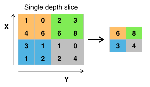
We can see here that we just take the maximum number in the pool and downsample the layer to contain that maximal number. Similarly an average pool would use the average of the numbers within the pooled group.
That was easy! We got the basics for the major topics in our paper that we needed to understand and we can start writing code.
Next we will build the model.